Optimizing query matching in the front-end

Optimizing front-performance: How re-thinking query representation lead to a 1000-fold performance increase.
Introduction to the Rentman API
The Rentman web application can be broken down into two main parts: the front-end, written in TypeScript and using the Angular framework, and the back-end, written in PHP. MySQL databases are used to store the data.
To facilitate communication between the front-end and back-end, we've build a non-standard CRUD API. The Rentman API features a JSON-based query language that allows for fine-grained control over the data that is returned, considering fields as well as the items themselves.
The simplest query would be an empty object ({}), which would return all items, given a specific type. A somewhat more complex query might look like this:
{
key: 'group',
value: 100,
comparator: '='
}
Given a planned equipment* item type, which has a group property, this would return all planned equipment in equipment group 100.
ⓘ In Rentman, equipment planned on a project is referred to as planned equipment. This equipment is usually split into equipment groups. Example equipment groups are: Sound, Lighting, Rigging, etc.
Front-end data handling
The query language is well suited to populating a view in the front-end. For instance, we might show a list of planned equipment items on a project page, constraining our list by using a query.
We refer to a set of items that can be described by a query as a collection. Available as a JavaScript object at runtime, a collection will often be referenced in an Angular component template. We leverage Angular changes detection to ensure the component is kept up to date whenever items are added to (or removed from) the collection.
Early on in the development of the Rentman front-end, we decided that we should have the ability to store changes client-side. When the user hits the save button, all client-side changes are aggregated and sent to the server.
This means, however, that a collection can contain remote items (originating from the server), as well as local items (originating from changes made by the user). For instance, when the user plans an additional piece of equipment on a project, this should influence our list of planned equipment items, even if the data is not stored on the server yet.
In order to facilitate this, we decided to introduce an abstraction layer where a collection can contain remote as well as local items.
Query matching
In the back-end, the API query is transformed to an SQL query, at which point the MySQL server takes care of returning the correct items. In the front-end, however, we don't have that luxury. That means that, given an API query, we need to discover:
- what newly created local items match the query;
- what locally updated remote items match the query;
- what locally updated remote items no longer match the query.
If we would, for example, match local items to the query described above, we would, for each local item in our cache:
- analyze the query;
- conclude we're dealing with a condition that is constraining the group field;
- look up the value of the group field of the respective item;
- carry out the required comparison.
However, using this approach, for n items and m queries, we'd have O(n*m) matching operations. As some projects would contain many equipment groups, each containing many planned equipment items, the number of operations would get quite large, and consequently, loading a view displaying those items would get quite slow.
For instance, we noticed that opening a particularly large project, containing over 9500 planned equipment items and 205 equipment groups, would take over half a minute! (This makes sense once you imagine the amount of matching operations would be approaching 2 million.)
Optimizing query matching
We were able to achieve significant performance benefits by changing the way we represent a query in the front-end. Instead of the JSON format that is used when doing a back-end request, we represent a query using rooted directed acyclic graph (DAG).
When transforming a query to a graph, a comparison will result in a comparator node, with the value being represented by an edge. Some example queries (and corresponding graphs) are listed below.
| ID | Query | Graph |
|---|---|---|
| 0 | {} | 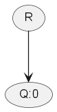 |
| 1 |
{ key: 'group', value: 100, comparator: '=' } |
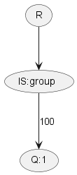 |
| 2 |
{ key: 'group', value: [200, 300], comparator: 'IN' } |
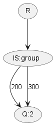
|
Graph merging
Up until now, each graph represents exactly one query. But we can do better: we can represent multiple queries using the same graph!
Suppose we have an item I, which is moved from group 100 to group 200. We'd like to match it against queries 1 and 2. If we merge the graphs of both queries, we can match the item using a single graph traversal.
A naïve way of merging the graphs would be:
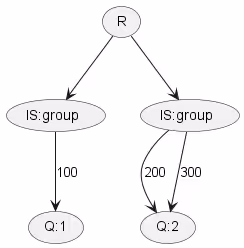
Note that the IS:group comparator node appears twice in the graph now. A better result would be:
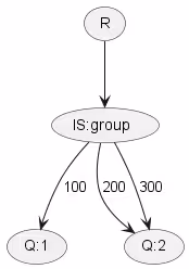
If we implement this effectively, we can now match the item to both queries using a single operation!
Graph matching
During the graph matching process, each node in the tree is represented by a class instance. We pass the fields of the item to the root node, as well as an accumulator variable to store results. We'd then traverse the tree to find out what queries would match this specific set of fields. (As opposed to our previous approach, where each query was matched to the fields individually.)
All comparator nodes (such as the IS:group node described above) have a match method. On a positive result, we then continue to traverse the subtree. When we reach a leaf node we store the associated match in the accumulator.
Note that the match function for the IS comparator nodes can be implemented effectively using a map.
Example
Suppose we have queries 0, 1 and 2, as well as item I, which is moved from group 100 to group 200. The graph representing these queries is:
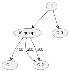
In order to discover the effect of this change, we need to traverse the graph twice: once with the previous value (100), and once with the current value (200).
The results would then be:
{
0: true,
1: true,
2: false
}
And:
{
0: true,
1: false,
2: true
}
Combining these results, we now know the item needs to be removed from the collection representing 1, and added to the collection representing 2.
Results
When tested on the project containing over 205 equipment groups and 9500 planned equipment items mentioned earlier, initial loading times went down from over half a minute to about 5 seconds. Time spent in the query matcher went down from about 28.000 milliseconds to about 20 milliseconds. That's three orders of magnitude faster!
Frequently asked questions

Previous blog posts